Still not convinced by Vicariance Biogeography

When reading recent methodological papers, review articles, or publications on my study group I sometimes add to the mix the odd paper that is not directly relevant for my work and maybe not even very recent but which is relevant to my broader interests. In this case I decided to take a look at Heads 2009, Inferring biogeographic history from molecular phylogenies, Biol J Linn Soc 98: 757-774.

Michael Heads is perhaps the most published proponent of Vicariance Biogeography, the school of biogeography that rejects speciation following long-distance dispersal (LDD) because... and that is where it gets interesting, because I still find that rejection puzzling. To the best of my understanding at least some vicariance biogeographers consider the conclusion of LDD to be unscientific because they believe it can explain any possible contemporary range, on the lines of 'if your hypothesis can explain every observation it explains nothing'. This does not make sense to me, because LDD would still be more or less plausible depending on the dating of cladogenesis events relative to tektonic events or island ages, prevailing wind and water currents, dispersal ecology, and many other factors. It also seems rather more unscientific to reject a possible explanation a priori, regardless of any evidence in its favour. But to get a better understanding of the arguments of vicariance biogeographers is precisely my reason for picking up this paper. So, on with it.

In a section titled "critique of founder dispersal in population genetic studies", Heads first describes the concept as "the founder individual has been isolated from its parent population by dispersing over a barrier (an apparent contradiction)". Right out of the gate this seems odd. I may be missing something, but it appears as if Heads would accept only extremes: either there is a barrier, meaning zero dispersal, or there is none, meaning panmixis. I have previously observed similar arguments in other papers from the vicariance school.

Assume I have a garden with a fence around it, and then one day a cat jumps over it. Does this mean I have no barrier around the garden? Of course not, it may still have kept various stray dogs and neighbours' children out. On the other hand, it was never a barrier to birds or insects. The same in biogeography. No barrier on this planet is absolute, and each barrier has a different force for different groups of organisms. A channel that is near-insurmountable to a monkey may be crossed by insects if blown over by a strong enough storm, and it may be no barrier at all to fern spores. Perhaps even more importantly, dispersal is a stochastic process. The Atlantic Ocean did not keep all cacti from crossing (Rhipsalis made it over to Africa), but it kept the seeds of >99.9% of them away, so it is still a barrier even if not an absolute one.

Beyond that the argument of the section relies on citing five papers that "failed to corroborate predictions of founder effect speciation", of which one is missing from the reference list. I checked three of the remaining four papers, and in all cases they are experiments on fruit flies limited to time frames on the order of ten years and designed to test the very narrow question whether severe population bottlenecks will cause pre-mating isolation. Now I may completely have misunderstood the claim made by mainstream biogeographers regarding founder speciation, but I believe it was not "ten years after an organism has dispersed to an island it will have achieved biological pre-mating isolation". The way I understand it the claim is more on the lines of the large distance from the parental population producing geographic pre-mating isolation, which enables speciation to take place subsequently. The point is not the speed with which the new population evolves (although that is an exciting research question in itself) but rather that it has become geographically isolated.

The argument consequently seems to miss the point. If there is a problem for founder speciation then it would be whether a single pregnant female or a single seed can establish a viable population. Potential problems are inbreeding and, in plants that have such features, self-incompatibility systems that cause failure to set seed. But if a population establishes, helped perhaps by herbivore release and lack of competition, subsequent speciation is not an extraordinary claim. It really does not matter if isolation has been achieved by vicariance or by LDD, the subsequent process of divergence is the same except the latter will also cause a genetic bottleneck.

The section "critique of founder dispersal in biogeographic studies" points out that there is good evidence for similar vicariance patters in many taxa. I am unaware of anybody who denies that vicariance is an important process - but it does not logically follow that LDD is therefor implausible. I can agree that a lot of white swans exist without therefore having to believe that black ones cannot possibly exist.

This is followed by "founder dispersal and new ideas on rift tectonics", where the idea seems to be that seemingly young oceanic islands do not require LDD to be colonised because they kind of have always been there. It is not entirely clear to me if the claim is that the individual islands are all much older than the oldest still observable lava flows or if, as implied by the reference to "seamounts", the local species would have constantly hopped from one short-lived and now submerged island to the next. If the first, it seems rather ad-hoc; if the second, one wonders why species that can so easily jump ten times from one disappearing island to the next island in the chain cannot simply jump a single time from continent to island. What is the more parsimonious conclusion here?

Next, molecular clocks and time calibration of phylogenies are rejected. All inferences, be it from fossils but in particular from geological events such as the formation of the isthmus of Panama, are dismissed as unreliable, but apparently present distributions are reliable evidence of ancestral distributions. Unfortunately I remain anti-convinced.

To quote the following paragraph in full:

"In Ronquist's (1997) method of dispersal-vicariance analysis, inferences of dispersal events are minimized as they attract a 'cost'. Extinction also attracts a cost but vicariance does not. It was not explained why this approach was taken and it appears to be based on a confusion of the two different concepts of 'dispersal'. Ecological dispersal in the sense of ordinary movement should not attract any cost in any model; founder dispersal would attract no cost in a traditional dispersalist model, but, in a vicariance model of speciation or evolution, it is rejected a priori."

What Heads does here is reject a formal parsimony-based inference of ancestral ranges in favour of, to judge from the second half of the paper, an informal, intuitive, pencil-on-a-map deduction process. What does he not like about Dispersal-Vicariance Analysis (DIVA)? Apparently primarily that dispersal events have a parsimony cost. It may be that he did not contemplate how such an analysis would work or if it could even work at all, if the only process having a cost would be extinction - of course it would mean that dispersal would be much too 'cheap', and every single ancestral species would always be inferred to have occupied the union of the ranges of its two descendants.

The great irony here is that even with a dispersal cost DIVA is well known for mercilessly (and implausibly) favouring vicariance as a process. I ran that analysis on two or three data sets a few years ago, and unless one restricts the maximum range size of ancestral species to something biologically plausible one pretty much always ends up with the vicariance biogeographers' preferred conclusion: the ancestor of the study group was already everywhere where any of its descendants occur today.

The second part of the paper is taken up by a large number of case studies, taxa which have sometimes been suggested to have undergone LDD but for which Heads presents a vicariance explanation instead. Some of these I find more plausible than others, but I do not want to go into each of them in detail. Instead, it seems more efficient to discuss what I see as three problems running through the entire argumentation:

First, there seems to be a lot of ad-hoccery going on. Where necessary to arrive at the conclusion of vicariance, for example to explain the overlapping distributions of African Arctotideae, 'normal ecological' range expansion is invoked as common and easy. But where necessary to arrive at the conclusion of vicariance, for example when distantly related subclades of a taxon occur right next to each other in Tasmania or New Zealand (suggesting relatively recent LDD from elsewhere), they are assumed to have been sitting in these narrow localities for tens of millions of years, apparently unable to move at all, so that a very ancient vicariance event can have taken place between their present ranges. Is that not rather convenient?

Which brings me to the second point. The text presenting the case studies certainly uses words like "may" and "might" a lot. To be honest, I sometimes found myself reminded of Erich von Daniken, whose style was to the effect of "the traditional explanation is that the pyramids were build by the ancient Egyptians - but could it not have been extra-terrestrials?" Yes, in each of these cases vicariance (or extra-terrestrials) could be the explanation. But mere possibility is a low hurdle to clear; the real question is, is that the most plausible explanation?

Third, as always with vicariance- or panbiogeography the problem is that dispersal is still required. Somehow this taxon here must have reached this volcanic island, somehow that taxon there must have spread all over the world. How does the vicariance biogeographer arrive at contemporary ranges without invoking jumps across oceans? Partly by hiding the dispersal away before the start of the analysis. To quote the present paper, "assuming a worldwide ancestor..." Well, if we can just assume that at our leisure it becomes easy to conclude few dispersal events, long distance or otherwise.

Now quite apart from the question whether a single species occurring worldwide is biologically realistic for all groups of organisms (I'd say it isn't), the problem remains that we have a lot of nested groups that would all have to have been ancestrally cosmopolitan, requiring several global range expansions in between. The daisy family is an excellent example. With reference to them, Heads writes that "through the history of the family as a whole, only a small number of widespread ancestors may have existed (groups such as Senecioneae and Astereae each require their own global ancestor)." I think that is a wee bit of an underestimate.

To walk through just one example in order of containing taxon to subordinate taxon: The Asteraceae family is cosmopolitan. The Asteroideae subfamily is cosmopolitan. The Astereae tribe is cosmopolitan. And the genus Conyza is cosmopolitan. If vicariance is the explanation for all speciation events we still need at least four consecutive cases of spreading across all continents. The same applies to a large number of the other tribes in the family: yes, that includes the aforementioned Senecioneae, but also Gnaphalieae, Anthemideae, Heliantheae, Cichorieae, Cardueae, Inuleae, and Vernonieae. And several of these include genera occurring across several continents or even (as with Senecio) all of them except Antarctica.

There is certainly a lot of dispersal required to explain that even in a vicariance approach, and unless we assume that most speciation in these groups took place before the breakup of Pangaea 175 million years ago (meaning the early dinosaurs would have known many of the same daisies as we do now, tens of millions of years before the oldest estimates for the origin of the daisy family) we will have to assume that some of that dispersal was long-distance.

Why not simply accept that organisms can sometimes, rarely but often enough to matter, cross an ocean and establish on the other side, followed by speciation? What is is so extraordinary about that conclusion, really? What is so different about it compared to being separated by vicariance, followed by speciation? I am still puzzled.

How problematic is the jump dispersal parameter in ancestral area inference?

I recently read an article in the Journal of Biogeography titled "Conceptual and statistical problems with the DEC + J model of founder-event speciation and its comparison with DEC via model selection". Its authors are Richard Ree, the developer of the original DEC model, and Isabel Sanmartin.

The main problem with discussing the paper here is that it would probably take 5,000 words to properly explain what it is even about. I will try to provide the most superficial introduction to the topic and otherwise assume that of the few people who will read this blog most are at least somewhat familiar with it.

The area of research this is about is the estimation or inference of ancestral areas and biogeographic events. Say we have a number of related species, the phylogeny showing how they are related, a number of geographic areas in which each species is either present or absent, and at least one model of biogeographic history. For the purposes of what I will subsequently call ancestral area inference (AAI) we assume that we know the species are well-defined and that the phylogeny is as close to true as we can infer at the time, so that they will simply be accepted as given. How to objectively define biogeographic areas for the study group is another big question, but again we take it as given that that has been done.

The idea of AAI is to take these pieces of information and infer what distribution ranges the ancestral species at each node of the phylogeny had, and what biogeographic events took place along the phylogeny to lead to the present patterns of distribution. What model of biogeographic events we accept matters a lot, of course. Imagine the following simple scenario of three species and three areas, with sister species occurring in areas A and B, respectively, and their more distant relative occurring in both areas B and C:



Assuming, for example that our model of biogeographic history favours vicariant speciation and range expansions, we may consider the scenario on the left to be a very probable explanation of how we ended up with those patterns of distribution. First the ancestral species of the whole clade occurred in all areas, and vicariant speciation split it into a species in area A and one in areas B and C. The former expanded to occur in both A and B and then underwent another vicariant speciation event, done.

If we have reason to assume that this is unlikely, for example because area A is an oceanic island, we may favour a different model. In the right hand scenario we see the ancestral species occurring in areas B and C and producing one of its daughter species via subset sympatry in area B. At least one seed or pregnant female of that new lineage is then dispersed to island A. An event such as this last one, where dispersal leads to instant genetic isolation and consequent speciation, is in this context often called 'jump dispersal' or, as in the title of the paper, 'founder-event speciation', to differentiate it from the much slower process of gradual range expansion followed by vicariant or sympatric speciation*.

I am not saying that either of these scenarios is the best one to explain how the hypothetical three species evolved and dispersed. In fact I would say that three species are too small a dataset to estimate biogeographic history with any degree of confidence, but it provides an idea of what ancestral area inference is about.

Perhaps the best established approaches to AAI are Dispersal and Vicariance Analysis (DIVA) and the Dispersal, Extinction and Cladogenesis model (DEC). The former was originally implemented as parsimony analysis in a software with the same name, and it has a tendency to favour vicariance, as the name suggests. Likelihood analysis under the DEC model became popular in its implementation in the software Lagrange, and in my limited experience and to the best of my understanding it is designed to have daughter species inherit part of the range of the ancestor, often leading to subset sympatry. And there are other approaches, of course.

As the result of his PhD project, Nick Matzke introduced the following two big innovations in AAI: First, the addition of a parameter j, for jump dispersal, to existing models. This allows the kind of instantaneous speciation after dispersal to a new area that I described above, and which can be assumed to be particularly important in island systems. Second, the idea that the most appropriate model for a study group should be chosen through statistical model selection, as in other areas of evolutionary biology. He created the R package BioGeoBEARS to allow such model selection. It implemented originally likelihood versions of DIVA, DEC and a third model called BayArea, all assuming the operation of slightly different sets of biogeographic processes. Each of them can be tested with and without the j parameter and, after another update, with or without an x parameter for distance-dependent dispersal.

Now I come finally (!) to Ree & Sanmartin. Their eight page paper, as the title implies, is a criticism of these two innovations. What do they argue? I hope I am summarising this faithfully, but in my eyes their three core points are as follows:

• A biogeographic model with events happening at the nodes of the tree as opposed to along the branches, as is the case with jump dispersal, is not a proper evolutionary model because such events are then "not modeled as time-dependent". In other words, only events that have a per-time-unit probability of occurring along a branch are appropriate.

• Under certain conditions the most probable explanation provided by a model including the j parameter is that all biogeographic events were jump dispersals. The j parameter gets maximised and explains everything by itself. They call this scenario "degenerate", because the "true" model must "surely" include time-dependent processes.

• DEC and DEC + j (and, I assume, by extension any other model and its + j variant) cannot be compared in the sense of model selection.

I must, of course, admit that model development is not my area. Consequently I am happy to defer regarding points one and three to others who have more expertise, and who will certainly have something to say about this at some point. I can only at this moment state that these claims do not immediately convince me. Certainly it is often the case that models with very different parameters are statistically compared with each other?

Is it not possible that the best model to explain an evolutionary process may sometimes indeed have a parameter that is not time-dependent but dependent on lineage splits? In the present case, if it is a fact that jump dispersal caused a lineage split, then both events quite simply happened instantaneously (at the relevant time scale of millions of years); in a sense, they were the same event, as the dispersal itself interrupted gene flow.

Perhaps more importantly, however, I am not at all convinced by the second point. Generally I am more interested in practical and pragmatic considerations than theory of statistics and philosophy. In phylogenetics, for example, I am less impressed by the claim that parsimony is supposedly not statistically consistent than by a comparison of the results produced by parsimony and likelihood analysis of DNA sequence datasets. Do they make sense? What can mislead an analysis? What software is available? How computationally feasible is what would otherwise be the best approach, and can it deal with missing data?

So in the present case I would also like to consider the practical side. Is the problem of j being maximised so that everything is explained by jump dispersal at all likely to occur in empirical datasets? In the paper Ree and Sanmartin illustrate a two species / two area example. That is clearly not a realistic empirical dataset, as it is much too small for proper analysis. But if we understand to some degree how the various model parameters work we can deduce under what circumstances j is likely to be maximised.

Unless I am mistaken, the circumstances appear to be as follows: We need a dataset in which all species are local endemics, i.e. all are restricted to a single area, and in which sister species never share part of their ranges. This is because other patterns cannot be explained by jump dispersal. If a species occupies two or more areas, it would have had to expand its range, so the analysis cannot reduce the d parameter for range expansion to zero. If sister species share part of their ranges, likewise; if they share the same single area, they must have diverged sympatrically, which again is not speciation through jump dispersal.

This raises the question, how likely are we to find datasets in which these two conditions apply? In my admittedly limited experience such datasets do not appear to be very common. If we are dealing, for example, with a small to medium sized genus on one continent, we will generally find partly overlapping ranges, and often at least one very widespread species. The j parameter will not be maximised. If we are doing a global analysis of a large clade, we will need rather large areas (because if you use too many small areas the problem becomes computationally intractable). This means, among other things, that entire subclades will share the same single-area range, and j will not be maximised.

In other words, the problem of 'all-jump dispersal' solutions appears to be rather theoretical. But what if we actually do have such a dataset? Is it not a problem then? To me the next question is under what circumstances such a situation would arise. Again, we have all species restricted to single areas, meaning that they apparently find it hard to expand their ranges across two areas. Why? Perhaps geographic separation to the degree that they rarely disperse? Geographic separation to the degree that when they disperse gene flow is interrupted, leading to immediate speciation? Again, we never have sister species sharing an area. Why? A good explanation would be that each area is too small for sympatric speciation to be possible.

Now what does that dataset sound like? To me it sounds like an archipelago of small islands, or perhaps a metaphorical island system such as isolated mountain top habitats. The exact scenario, in other words, in which all-jump dispersal seems like a very probable explanation. Because your ancestral island is too small for speciation, the only way to speciate is to jump to another island, and if you jump to another island you are immediately so isolated from your ancestral population that you speciate.

Again, I am not a modeler, and I have not run careful simulation experiments before writing this, but based on this thought experiment it seems to me as if the + j models would work just as they should: j would not be maximised under circumstances where the other processes are needed to explain present ranges, but it would be maximised under precisely those extremely rare circumstances where 'all jump dispersal' is the only realistic explanation.

Footnote

*) Sympatric meaning here at the scale of the areas defined for the analysis. If one the areas in the analysis is all of North America, for example, it is likely that the 'sympatric' events inside that area would in truth mostly have been allopatric, parapatric or peripatric at a smaller spatial scale.

Bioregionalisation part 6: Modularity Analysis with the R package rnetcarto

Today's final post in the bioregionalisation series deals with how to do a network or Modularity Analysis in R. There are two main steps here. First, because we are going to assume, as in the previous post, that we have point distribution data in decimal coordinates, we will turn them into a bipartite network of species and grid cells.

We start by defining a cell size. Again, our data are decimal coordinates, and subsequently we will use one degree cells.

cellsize <- 1

Note that this may not be the ideal approach for publication. The width of one degree cells decreases towards the poles, and in spatial analyses equal area grid cells are often preferred because they are more comparable. If we want equal area cells we first need to project our data into meters and then use a cellsize in meters (e.g. 100,000 for 100 x 100 km). There are R functions for such spatial projection, but we will simply use one degree cells here.

We make a list of all species and a list of all cells that occur in our dataset, naming the cells after their centres in the format "126.5:-46.5". I assume here that we have the data matrix called 'mydata' from the previous post, with the columns species, lat and long.

allspecies <- unique(mydata$species)

longrounded <- floor(mydata$long / cellsize) * cellsize + cellsize/2

latrounded <- floor(mydata$lat / cellsize) * cellsize + cellsize/2

cellcentre <- paste(longrounded,latrounded, sep=":")

allcells <- unique(cellcentre)

We create a matrix of species and cells filled with all zeroes, which means that the species does not occur in the relevant cell. Then we loop through all records to set a species as present in a cell if the coordinates of at least one of its records indicate such presence.

mynetw <- matrix(0, length(allcells), length(allspecies))
for (i in 1:length(mydata[,1]))
{
  mynetw[ match(cellcentre[i],allcells) , match(mydata$species[i], allspecies) ] <- 1
}

It is also crucial to name the rows and columns of the network so that we can interpret the results of the Modularity Analysis.

rownames(mynetw) = allcells
colnames(mynetw) = allspecies

Now we come to the actual Modularity Analysis. We need to have the R library rnetcarto installed and load it.

library(rnetcarto)

The command to start the analysis is simply:

mymodules <- netcarto(mynetw, bipartite=TRUE)

This may take a bit of time, but after talking to colleagues who have got experience with other software it seems it is actually reasonably fast - for a Modularity Analysis.

Once the analysis is done, we may first wonder how many modules, which we will subsequently interpret as bioregions, the analysis has produced.

length(unique(mymodules[[1]]$module))

For publication we obviously want a decent map, but that is beyond the scope of this post. What follows is merely a very quick and dirty way of plotting the results to see what they look like, but of course the resulting coordinates and module numbers can also be used for fancier plotting. We split the latitudes and longitudes back out of the cell names, define a vector of colours to use for mapping (here thirteen; if you have more modules you will of course need a longer vector), and then we simply plot the cells like some kind of scatter plot.

allcells2 <- strsplit( as.character( mymodules[[1]]$name ), ":" )

allcells_x <- as.numeric(unlist(allcells2)[c(1:(length(allcells)))*2-1])
 
allcells_y <- as.numeric(unlist(allcells2)[c(1:(length(allcells)))*2])
 
mycolors <- c("green", "red", "yellow", "blue", "orange", "cadetblue", "darkgoldenrod", "black", "darkolivegreen", "firebrick4", "darkorchid4", "darkslategray", "mistyrose")

plot(allcells_x, allcells_y, col = mycolors[ as.numeric(mymodules[[1]]$module) ], pch=15, cex=2)

There we are. Modularity analysis with the R library rnetcarto is quite easy, the main problem was building the network.

As an example I have done an analysis with all Australian (and some New Guinean) lycopods, the dataset I mentioned in the previous post. It plots as follows.

There are, of course, a few issues here. The analysis produced six modules, but three of them, the green, orange and light blue ones, consist of only two, one and one cells, respectively, and they seem biologically unrealistic. They may be artifacts of not having cleaned the data as well as I would for an actual study, or represent some kind of edge effect. The remaining three modules are clearly more meaningful. Although they contain some outlier cells, we can start to interpret them as potentially representing tropical (red), temperate (yellow), and subalpine/alpine (dark blue) assemblies of species, respectively.

Despite the less than perfect results I hope the example shows how easy it is to do such a Modularity Analysis, and if due diligence is done to the spatial data, as we would do in an actual study, I would also expect the results to become cleaner.

Bioregionalisation part 5: Cleaning point distribution data in R

I should finally complete my series on bioregionalisation. What is missing is a post on how to do a network (Modularity) analysis in R. But first I thought I would write a bit about how to efficiently do some cleaning of point distribution data in R. As often I write this because it may be useful to somebody who finds it via search engine, but also because I can then look it up myself if I need it after not having done it for months.

The assumption is that we start our spatial or biogeographic analyses by obtaining point distribution data by querying e.g. for the genus or family that we want to study on an online biodiversity database or aggregator such as GBIF or Atlas of Living Australia. We download the record list in CSV format and now presumably have a large file with many columns, most of them irrelevant to our interests.

One problem that we may find is that there are numerous cases of records occurring in implausible locations. They may represent geospatial data entry errors such as land plants supposedly occurring in the ocean, or vouchers collected from plants in botanic gardens where the databasers fo some reason entered the garden's coordinates instead of those of the source location , or other outliers that we suspect to be misidentifications. What follows assumes that this at least has been done already (and it is hard to automate anyway), but we can use R to help us with a few other problems.

We start up R and begin by reading in our data, in this case all lycopod records downloaded from ALA. (One of the advantages about that group is that very few of them are cultivated in botanic gardens, and I did not want to do that kind of data clean-up for a blog post.)

rawdata <- read.csv("Lycopodiales.csv", sep=",", na.strings = "", header=TRUE, row.names=NULL)

We now want to remove all records that lack any of the data we need for spatial and biogeographic analyses, i.e. identification to the species level, latitude and longitude. Other filtering may be desired, e.g. of records with too little geocode precision, but we will leave it at that for the moment. In my case the relevant columns are called genus, specificEpithet, decimalLatidue, and decimalLongitude, but that may of course be different in other data sources and require appropriate adjustment of the commands below.

rawdata <- rawdata[!(is.na(rawdata$decimalLatitude) | rawdata$decimalLatitude==""), ]
rawdata <- rawdata[!(is.na(rawdata$decimalLongitude) | rawdata$decimalLongitude==""), ]
rawdata <- rawdata[!(is.na(rawdata$genus) | rawdata$genus==""), ]
rawdata <- rawdata[!(is.na(rawdata$specificEpithet.1) | rawdata$specificEpithet.1==""), ]

All the records missing those data should be gone now. Next we make a new data frame containing only the data we are actually interested in.

lat <- rawdata$decimalLatitude
long <- rawdata$decimalLongitude
species <- paste( as.character(rawdata$genus), as.character(rawdata$specificEpithet.1, sep=" ") )
mydata <- data.frame(species, lat, long)
mydata$species <- as.character(mydata$species)

Unfortunately at this stage there are still records that we may not want for our analysis, but they can mostly be recognised by having more than the two usual name elements of genus name and specific epithet: hybrids (something like "Huperzia prima x secunda" or "Huperzia x tertia") and undescribed phrase name taxa that may or may not actually be distinct species ("Lycopodiella spec. Mount Farewell"). At the same time we may want to check the list of species in our data table with unique(mydata$species) to see if we recognise any other problems that actually have two name elements, such as "Lycopodium spec." or "Lycopodium Undesignated". If there are any of those, we place them into a vector:

kickout <- c("Lycopodium spec.", "Lycopodium Undesignated")

Then we loop through the data to get rid of all these problematic entries.

myflags <- rep(TRUE, length(mydata[,1]))
for (i in 1:length(myflags))
{
  if ( (length(strsplit(mydata$species[i], split=" ")[[1]]) != 2) || (mydata$species[i]) %in% kickout )
  {
    myflags[i] <- FALSE
  }
}
mydata <- mydata[myflags, ]

If there is no 'kickout' vector for undesirable records with two name elements, we do the same but adjust the if command accordingly to not expect its existence.

Check again unique(mydata$species) to see if the situation has improved. If there are instances of name variants or outdated taxonomy that need to be corrected, that is surprisingly easy with a command along the following lines:

mydata$species[mydata$species == "Outdatica fastigiata"] = "Valida fastigiata"

In that way we can efficiently harmonise the names so that one species does not get scored as two just because some specimens still have an outdated or misspelled name.

Although we assume that we had checked for geographic outliers, we may now still want to limit our analysis to a specific area. In my case I want to get rid of non-Australian records, so I remove every record outside of a box of 9.5 to 44.5 degrees south and 111 to 154 degrees east around the continent. Although it turns out that this left parts of New Guinea in that is fine with me for present purposes, we don't want to over-complicate this now.

mydata <- mydata[mydata$long<154, ]
mydata <- mydata[mydata$long>111, ]
mydata <- mydata[mydata$lat>(-44.5), ]
mydata <- mydata[mydata$lat<(-9.5), ]

At this stage we may want to save the cleaned up data for future use, just in case.

write.table(mydata, file = "Lycopodiales_records_cleaned.csv", sep=",")

And now, finally, we can actually turn the point distribution data into grid cells and conduct a network analysis, but that will be the next (and final) post of the series.

Alpha diversity and beta diversity

At today's journal club meeting, we discussed Alexander Pyron's opinion piece We don't need to save endangered species - extinction is part of evolution. I mentioned it in passing before and still think that his core argument, which is also reflected in the title, is logically equivalent to saying that murder is okay because all humans are going to die of natural causes one day anyway. But reading his piece more thoroughly than before, I now notice a few other, um, problems. The highlights:

Species constantly go extinct, and every species that is alive today will one day follow suit. There is no such thing as an "endangered species," except for all species.

What weirds me out here is the lack of a phylogenetic perspective in a piece written by a systematist - species are discussed as individuals that pop out of thin air and then disappear again. Of course, in the very long run every species will one day go extinct when the sun expands and boils off the oceans. But until then, in the time frame that Pyron discussed, no, not every species will go extinct, quite a few of them will diversify and survive as numerous descendant species, as did the ancestor of all land vertebrates or the ancestor of all insects in the past. They thus become effectively immortal (until, once more, the sun explodes anyway, etc.).

Yet we are obsessed with reviving the status quo ante. The Paris Accords aim to hold the temperature to under two degrees Celsius above preindustrial levels, even though the temperature has been at least eight degrees Celsius warmer within the past 65 million years. Twenty-one thousand years ago, Boston was under an ice sheet a kilometer thick. We are near all-time lows for temperature and sea level ; whatever effort we make to maintain the current climate will eventually be overrun by the inexorable forces of space and geology.

This is sadly a classic of climate change denialism. Yes, there was change in the past too, but there are some major differences. One is the rate of change - the impacts we are having are coming much faster than most natural changes (excepting e.g. meteorite strikes and similarly sudden events), so that animals and plants have less of a chance to migrate or to adapt than they had in past cycles of warm and ice ages. Second, they have even less of a chance to migrate because we have fragmented their available habitats by putting roads, towns, croplands and pastures into their way. Third, past changes did not affect a highly urbanised human population of more than seven billion people; the potential of global change producing catastrophic results even just for us is much greater now than when we were just a few million widely dispersed hunter-gatherers. So yes, it is true that we cannot freeze the status quo in place forever, but I think we would do well to slow the rate of change as far as possible.

Infectious diseases are most prevalent and virulent in the most diverse tropical areas. Nobody donates to campaigns to save HIV, Ebola, malaria, dengue and yellow fever, but these are key components of microbial biodiversity, as unique as pandas, elephants and orangutans, all of which are ostensibly endangered thanks to human interference.

I just don't even. What is the logic here? "Nobody cares about conserving diseases that horribly kill us humans, so we should not care about conserving harmless pandas either?" How does that follow?

And if biodiversity is the goal of extinction fearmongers, how do they regard South Florida, where about 140 new reptile species accidentally introduced by the wildlife trade are now breeding successfully? No extinctions of native species have been recorded, and, at least anecdotally, most natives are still thriving. The ones that are endangered, such as gopher tortoises and indigo snakes , are threatened mostly by habitat destruction. Even if all the native reptiles in the Everglades, about 50, went extinct, the region would still be gaining 90 new species -- a biodiversity bounty. If they can adapt and flourish there, then evolution is promoting their success. If they outcompete the natives, extinction is doing its job.

And this is perhaps what frustrates me most, because while this is not an uncommon argument against biosecurity measures one would expect a biologist to know about different types of biodiversity instead of confusing them. To explain more clearly what is going on, consider the following diagrams. First, we have three areas, roundland, squareland, and hexagonland, with two endemic species each.

Then humans recklessly move species between the areas, allowing them to invade each other's natural ranges. It turns out that three of the species are particularly competitive and prosper at the cost of the other three, driving them to extinction.

Now there are three types of diversity to consider. The first is alpha-diversity, which means simply the number of species in a given place. As we see it has gone up by 50% in all three areas, from two to three species. Yay, more diversity! This is what Pyron proudly points at in Florida.

What is lost, however, is beta-diversity or turnover, that is the heterogeneity you observe as you move between areas. It was very high originally, as every area had its unique species, but now it has been wiped out entirely. Beta-diversity in the second diagram is precisely zero. Under the first scenario a squarelander can go on a holiday trip to roundland and admire the unique flora of that part of the world; under the second scenario they will travel to roundland and merely see the same few weeds that they have growing in their own front yard back home. And the endemic plants of hexagonland have all gone extinct, a 100% loss of that area's irreplaceable evolutionary history.

(Note that beta-diversity would also be zero if all six species survived everywhere. But that is clearly not a realistic assumption, as it would require each area to have such a high carrying capacity that they should each have evolved more than two species to begin with. We would not expect that all the plant species of the world could survive next to each other in, say, Patagonia, even if they were all introduced there.)

Finally, in our example global diversity has of course also been reduced, by 50%. So yeah, great to have more alpha-diversity in Florida, but does that make up for a massive net loss in both beta-diversity and global diversity? The argument seems rather misguided.

Bioregionalisation part 4: networks

Having examined a clustering approach to bioregionalisation, today I will try to illustrate the increasingly popular alternative of network analysis.

Consider again our hypothetical study area of five cells with five taxa, where we want to know how to delimit bioregions (or phytoregions, given that the taxa are plant species) in an objective way:

The first step in the analysis is to interpret these data as a network. Specifically, as we have two different types of elements, what we are dealing with is called a bipartite network. Each type of element is connected directly only to elements of the other type, and to elements of its own type only via the other. In this case, the plant species are connected to all cells they occur in, and cells are connected to all plant species occurring in them:

Once we have scored this kind of network structure in a way that the software of our choice understands (either a list of connections or a matrix with 0s and 1s), we can use an algorithm that divides the network into modules. This algorithm tries to maximise connections within a module and to minimise the connections between modules, which in bioregion terms again means to maximise endemism.

As indicated in the posts on clustering, network analysis has the great advantage that it does not only produce groups, it also provides a reproducible and objective answer for the question about the optimal number of groups, whereas in clustering analysis the user still has to make a subjective decision.

That being said, it is always possible to take a large module by itself and explore its internal structure, if so desired, although of course the answer may be that there are no meaningful subdivisions any more.

Either way, any such algorithm will return modules, and what we are mostly interested in is what cells belong to what module. Nonetheless we would also be able to infer what species belong to what module, and depending on the type of network analysis we may be able to get other statistics that may be of interest for the network and for each individual module or even each element.

There are two main approaches to network analysis that have been explored in bioregionalisation. The first is called the Map Equation, developed by Rosvall et al. (2009) and promoted with a sleek, eponymous website. It was first applied to bioregionalisation by Vilhena & Antonelli (2015). One of its advantages is that it is the faster of the two, which may be particularly attractive if one's dataset is large and complex.

The second is Modularity Analysis (Newman, 2006). This is the approach that I prefer personally, after colleagues at my institution conducted a study comparing the two and clustering against each other (Bloomfield et al., 2017). It is slower than the Map Equation, but it seems to be better at recognising the transitional nature of cells situated between two 'pure' modules, which the Map Equation appears to tend to group into distinct modules in their own right.

Next time, how to do modularity analysis in practice.

References

Bloomfield NJ, Knerr N, Encinas-Viso F, 2017. A comparison of network and clustering methods to detect biogeographical regions. Ecography 41: 1-10.

Newman MEJ, 2006. Modularity and community structure in networks. Proceedings of the National Academy of Sciences, USA 103: 8577-8582.

Rosvall M, Axelsson D, Bergstrom CT, 2009. The map equation. arXiv: 0906.1405 [physics.soc-ph]

Vilhena DA, Antonelli A, 2015. A network approach for identifying and delimiting biogeographical regions. Nature Communications 6: 6848.

Bioregionalisation part 3: clustering with Biodiverse

Biodiverse is a software for spatial analysis of biodiversity, in particular for calculating diversity scores for regions and for bioregionalisation. As mentioned in previous posts, the latter is done with clustering. Biodiverse is freely available and extremely powerful, just about the only minor issues are that the terminology used can sometimes be a bit confusing, and it is not always easy to intuit where to find a given function. As so often, a post like this might also help me to remember some detail when getting back to a program after a few months or so...

The following is about how to do bioregionalisation analysis in Biodiverse. First, the way I usually enter my spatial data is as one line per sample. So if you have coordinates, the relevant comma separated value file could look something like this:

species,lat,long
Planta vulgaris,-26.45,145.29
Planta vulgaris,-27.08,144.88
...

To use equal area grid cells you may have reprojected the data so that lat and long values are in meters, but the format is of course the same. Alternatively, you may have only one column for the spatial information if your cells are not going to be coordinate-based but, for example, political units or bioregions:

species,state
Planta vulgaris,Western Australia
Planta vulgaris,Northern Territory
...

Just for the sake of completeness, different formats such as a tsv would also work. Now to the program itself. You are running Biodiverse and choose 'Basedata -> Import' from the menus.

Navigate to your file and select it. Note where you can choose the format of the data file in the lower right corner. Then click 'next'.

The following dialogue can generally be ignored, click 'next' once more.

But the third dialogue box is crucial. Here you need to tell Biodiverse how to interpret the data. The species (or other taxa) need to be interpreted as 'label', which is Biodiversian for the things that are found in regions. The coordinates need to be interpreted as 'group', the Biodiversian term for information that defines regions. For the grouping information the software also needs to be told if it is dealing with degrees for example, and what the size of the cells is supposed to be. In this case we have degrees and want one degree squared cells, but we could just as well have meters and want 100,000 m x 100,000 m cells.

After this we find ourselves confronted with yet another dialogue box and learn that despite telling Biodiverse which column is lat and which one is long it still doesn't understand that the stuff we just identified as long is meant to be on the x axis of a map. Arrange the two on the right so that long is above lat, and you are ready to click OK.

The result should be something like this: under a tab called 'outputs' we now have our input, i.e. our imported spatial data.

Double-clicking on the name of this dataset will produce another tab in which we can examine it. Clicking on a species name will mark its distribution on the map below. Clicking onto a cell on the map will show how similar other cells are to it in their species content. This will, of course, be much less clear if your cells are just region names, because in that case they will not be plotted in a nice two-dimensional map.

Now it is time to start our clustering analysis. Select 'Analyses -> cluster' from the menu. A third tab will open where you can select analysis parameters. Here I have chosen S2 dissimilarity as the metric. If there are ties during clustering it makes sense to break them by maximising endemism (because that is the whole point of the analysis anyway), so I set it to use Corrected Weighted Endemism first and then Weighted Endemism next if the former still does not resolve the situation. One could use random tie-breaks, but that would mean an analysis is not reproducible. All other settings were left as defaults.

After the analysis is completed, you can have the results displayed immediately. Alternatively, you can always go back to the first tab, where you will now find the analysis listed, and double-click it to get the display.

As we can see there is a dendrogram on the right and a map on the left. There are two ways of exploring nested clusters: Either change the number of clusters in the box at the bottom, or drag the thick blue line into a different position on the dendrogram; I find the former preferable. Note that if you increase the number too much Biodiverse will at a certain point run out of colours to display the clusters.

The results map is good, but we you may want to use the cluster assignments of the cells for downstream analyses in different software or simply to produce a better map somewhere else. How do you export the results? Not from the display interface. Instead, go back to the outputs tab, click the relevant analysis name, and then click 'export' on the right.

You now have an interface where you can name your output file, navigate to the desired folder, and select the number of clusters to be recognised under the 'number of groups' parameter on the left.

The reward should be a csv file like the following, where 'ELEMENT' is the name of each cell and 'NAME' is the column indicating what cluster each cell belongs to.

Again, very powerful, only have to keep in mind that your bioregions, for example, are variously called clusters, groups, and NAME depending on what part of the program you are dealing with.

Bioregionalisation part 2: clustering

Already I think I should change the way I was going to do this. It seems more straightforward to keep the two approaches in separate posts. So for today: bioregionalisation using clustering methods.

A small example

As the term clustering suggests the approach is very simple. Let's start by considering a landscape of five cells A-E with five species occurring in them as follows:

Another way of expressing this information is as a matrix where the cells are rows and the species are columns, and presence of a species is indicated with "1" while absence is indicated with "0":

We now simply calculate a distance matrix. There are several possible dissimilarity metrics we can use for this. For this post I will use the S2 dissimilarity, which is defined as

S2 dissimilarity = 1 - ( number of shared species / ( number of shared species + minimum( species unique to first cell , species unique to second cell ) ) )

The resulting S2 dissimilarity matrix for our small dataset is consequently as follows:

Now we use a hierarchical clustering algorithm to produce a dendrogram. I have used R's hclust, and the result is:

We can now recognise clusters as bioregions, and we are done. The main remaining problem with hierarchical clustering is that there is no objective answer for the number of bioregions we should recognise. We could still accept anywhere between one and five, but at least we know that there should not be a region of e.g. only the cells C and E to the exclusion of D.

(This is of course the same problem as in phylogenetic systematics, where we would now know that CE to the exclusion of D is not an acceptable taxon, but it remains a subjective decision whether to recognise CD and E as separate genera or whether to have one genus CDE, for example.)

In our present, case it seems sensible to accept less than five regions but more than one, otherwise we would not have needed the analysis, so let's go with the two clusters AB and CDE:

These regions now show a fairly high level of endemism, as four of the five species are endemic to one region; only the blue species occurs across both.

Some R code

Although the proper software for this kind of work is Biodiverse, this post would get too long if I tried to do everything in one go. What is more, a simple analysis can just as well be run in R, which is what I have done in this case. First build a matrix of cells and the species in them, e.g.

occurs <- as.matrix(rbind(c(1,1,0,0,0), c(1,1,1,0,0), c(0,0,1,1,0), c(0,0,1,1,0), c(0,0,0,1,1)))
rownames(occurs) <- c("A", "B", "C", "D", "E")
colnames(occurs) <- c("red","brown","blue","orange","lilac")

The following loops will then produce a matrix of S2 dissimilarity scores.

mydm <- matrix(0, 5, 5)    # create empty matrix; could make it more flexible for future analyses by handing over square root of length(occurs) for the dimensions
rownames(mydm) <- c("A","B","C","D","E")    # same here, could use row names from occurs
colnames(mydm) <- c("A","B","C","D","E")     # and same here
for (i in 1:5)
{
  for (j in i:5)
  {
    if (i==j)
    {
      mydm[i,j] <- 0
    }
    else
    {
      shareds <- sum(occurs[i,] & occurs[j,])
      uniques_i <- sum(xor(occurs[i,], occurs[i,] & occurs[j,]))
      uniques_j <- sum(xor(occurs[j,], occurs[i,] & occurs[j,]))
      mydm[i,j] <- 1- (shareds / (shareds + min( uniques_i, uniques_j)))
      mydm[j,i] <- mydm[i,j]
    }
  }
}

Now finally do a cluster analysis and plot the resulting dendrogram:

mycl <- hclust(as.dist(mydm), method = "mcquitty")     # WPGMA
plot(mycl)

Done. For large numbers of cells we would want a decent visualisation, ideally as a map, and that is where Biodiverse works better. How to do the analysis in that software will be covered in the next post.

Bioregionalisation part 1: what's the idea?

This is the start of a little series of posts on bioregionalisation. I intend to divide the topic up as follows:

1. What I mean with bioregionalisation and what it is good for.
2. Comparison of two different quantitative approaches to defining bioregions, clustering and network analysis.
3. Practical how-to guide to inferring bioregions with clustering in the software Biodiverse.
4. Practical how-to guide to inferring bioregions with network analysis in R.
5. Beyond species presence and absence, i.e. using phylogenies for bioregionalisation.

Let's see if that works. So today:

What do I mean with bioregionalisation?

The idea is to divide a study region - perhaps a country, a continent or the whole world - into natural regions. There are obviously lots of different ways of doing so. A well-known one is climatic, where we would have arctic, temperate, subtropical, and tropical regions. Closer to what I am talking about are vegetation zones; in this case the general appearance of the natural vegetation and the life form of its constituent species are used to define zones such as tundra, boreal forest, mallee, or savanna.

But that still is not what this is going to be about. The bioregions I am going to discuss are defined by the taxa that occur in them. A very high-level classification is shown, for example, in the following map from earthonlinemedia.com:

As we can see there are no 'tropics', but instead the American tropics are separated from the African and South Asian ones. Why might that be the case? As a botanist I can immediately think of two important plant families that are very characteristic of the Neotropics but are (with the exception of one rather odd, small genus) entirely missing from the Paleotropics: the cactus family Cactaceae and the pineapple family Bromeliaceae.

This, then, is what bioregions as I will subsequently discuss them are: they are regions defined by the presence of (plant, animal, ...) taxa they do not share with other regions. Another way of putting it is that bioregionalisation aims to maximise the endemism of its regions. And this immediately suggests the possibility of quantitative, objective analyses as long as we can somehow quantify endemism.

But these approaches are for other posts. More importantly now:

Why do we care? What are these bioregions good for?

I can think of at least two use cases. The first is quite simply that we like to classify things, and climate and vegetation form do not capture all there is to natural regions. Specifically, the presence e.g. of bromeliads, leaf cutter ants and hummingbirds in the New World and their absence in the Old World is an accident of history that is orthogonal to the shared climate and to the fact that 'tropical rainforest' kind of looks the same from a distance in all continents. But it still matters because these groups of organisms have evolved unique characteristics, like the hummingbirds' high metabolic rate, that have an ecological impact. A neotropical cloud forest 'works' a bit differently than a southeast Asian one.

The second use case is that of finding objectively defensible regions for biogeographic analysis, a problem that still does not have a single widely accepted solution. For example, we may be interested in conducting an inference of ancestral areas and biogeographic processes using the R package BioGeoBears, because we want to know if our study group started evolving in the temperate part of our continent and then spread into the tropics or vice versa. For this analysis we need (a) a time-calibrated phylogeny and (b) a data table of taxa-by-regions showing for each region what taxa are naturally occurring in them.

Taking one step back, it is obvious then that we first need to define regions. This may be easy if we can simply use the islands of an island group, but taking a big blob of land like Australia as an example, how do we cut that up? States? Clearly political units are kind of iffy for biogeography, because they are human inventions. Climate or vegetation zones are more natural, but are they meaningful for our specific study group? How meaningful would a region be for my purposes that happens to have one of my study taxa scored as present because it comes in from the side into 5% of that region's extent?

To me at least it seems as if the solution is bioregionalisation by taxon content: take small units like 100 x 100 km cells or similar and use an objective bioregionalisation approach to group them into meaningful larger regions. As mentioned above this maximises endemism, which is precisely what I would want for the inference of ancestral areas and biogeographic history.

Having fun with biodiversity databases

If you have ever professionally used a biodiversity database you will soon have noticed that we still have a long way to go before they are as reliable as we would like them to be.

Today I looked into the Atlas of Living Australia records for Senecio australis (Asteraceae). Except for a rather odd specimen from South Africa the distribution records look like this:

What do we have here? First, the four Australian mainland records all appear to be misapplications of the name. The Flora of New South Wales, for example, does not even mention the species, so I think we can safely assume it does not occur in Australia at all.

Second, the record in the middle of the top of the map is right in the ocean, no matter how closely we zoom in. If we look into its details, we see that it was collected on Norfolk Island, which is the cluster of red dots to its right, so somebody must have got the coordinates rather wrong.

Third, there is a cluster around Auckland, on New Zealand's North Island. I am not sure if Norfolk Island and North Island is a plausible area of distribution for this species, but it may well be. Zooming in closer to Norfolk Island, however, ...

... it looks as if somebody had played darts after having had a few too many beers. ALA informs us dryly under the section data quality tests, "habitat incorrect for species". No kidding. Or as my wife joked, unwilling to believe that the coordinates would be so badly off for such a large percentage of the specimens, "is there a fish that is also called Senecio australis?"

These are the problems that we are dealing with, more generally.

• Whenever we do a study using data from biodiversity databases, as we increasingly do, we have to be very careful about cleaning the data. The main issues are outdated taxonomy, misidentifications, spatial data entry errors (which are particularly easy to recognise if an outlier record is exactly ten degrees away from a known occurrence), and imprecise spatial data. Just think of what it would do to species distribution modeling if we uncritically accepted all the records for Senecio australis.

• While we can identify obvious mistakes while using a database, the data are "ground-truthed" in the actual specimens in some herbarium or museum, and the policy is usually (and quite sensibly) that the database won't update until a correction is made to that specimen in its home institution and then filters through from there. But many institutions do not have the resources to update data just because somebody sent them an eMail pointing out that their specimen is misidentified or that they made a data entry error; many herbaria on the planet are so understaffed that even the word understaffed is a euphemism. What is more, even if a database allows a registered user to annotate a record with corrections, the information may not necessarily flow back to the institution holding it, depending on whether somebody thought to set up such procedures or not.

• Overall, Australia actually has excellent data quality, the Atlas of Living Australia actually allows annotations to be made, and several important Australian herbaria actually have the staffing to update their data. What I am saying is that this is as good as you can have it at the moment. It is much more difficult in many other parts of the world, and of course it would be good if we could have the same or better data quality for those areas.

Also, perhaps it is best not think too much about records that are not specimen-based but "human observations" or photos submitted by random people. There are, obviously, non-taxonomists whose knowledge of the flora is extensive, and citizen science can be awesome, but I have also seen several cases one the lines of "aaargh ... this is so misidentified it is not even the right tribe of the family, and now the database is using it as the profile picture of this nationally significant weed species!"

I still don't get area cladistics, and 'geographic paralogy' in particular

Since I started looking into panbiogeography and area cladistics, I have been curious about the concept of geographic paralogy. The word is used by area cladists (in the widest sense), and I have so far been doubtful about whether the analogy to gene paralogy fits.

To recap, area cladistics attempts to infer biogeographic area relationships from the patterns that species' areas of distribution show on a phylogenetic tree. If, for example, several plant or animal groups show distributions on a phylogeny that are ( Africa, ( South America , Australia ) ), i.e. sister lineages are endemic to South America and Australia, and more distantly related lineages are endemic to Africa, then an area cladist would conclude that South America and Australia are "more closely related" biogeographically than either is to Africa, or even that they form a "monophyletic biogeographic area".

Whatever that is supposed to mean, given that the word monophyletic only applies if we presuppose tree-like relationships. But I am getting ahead of myself.

The problem is now that phylogenies do not necessarily show such a simple pattern. Some species may be widespread and occur in several of the areas in the analysis, and of course the same area may occur repeatedly in different parts of the phylogeny. This is what area cladists call 'geographic paralogy', and they 'solve' the problem it poses for their analyses by selecting 'paralogy-free' subtrees from a phylogeny.

Again, two questions: Does it make sense to call this geographic paralogy, in analogy to gene paralogy? And does it make sense to do area cladistics by cherry-picking 'paralogy-free' subtrees, effectively ignoring these patterns?

I started a conversation with a colleague at the IBC, and he recommended I read Ladiges (1998, "Biogeography after Burbidge", Australian Systematic Botany 11: 231-242) as an introduction to the relevant concepts and approaches. So this I have now done. Unfortunately, the paper did not really solve my conceptual problems. I will start with a few quotes:

In cladistic biogeography, nodes of a cladogram for organisms (1,2 and 3) are potentially informative about the geographic areas (A, B and C) in which they occur: node 2 in Fig. 3 shows that areas B and C are related more closely to each other than to area A.

Such statements of relationship, the nodes of the cladogram, are explained by a variety of historical theories. One is dispersal from a restricted ancestral area, for example from area A to areas B and C, a pattern that may match fossil ages and distribution. An alternative explanation is vicariance of a widespread ancestral species coincident with physical breakup or climatic differentiation of the general area. A vicariance explanation is favoured by evidence of biogeographic congruence: finding the same pattern for other groups of organisms.

So far so good, although I do wonder whether the concept of area relationships makes sense if dispersal is the right answer. It seems to me that even calling it relationships only makes sense if there is no frequent floristic or faunal exchange, if near-everything is due to vicariance. And as I have mentioned before, there are good alternative explanations for congruence that do not imply vicariance, in particular prevailing directions of wind or ocean currents, common routes of migratory birds, etc.

Now come the complications:

Data for any one group of organisms are rarely as simple as the example shown (...). Some taxa are widespread, and some areas have more than one taxon. When combining data for different groups of organisms, not all areas are represented in each taxonomic group. Such complications are obstacles to development of analytical methods for determining area cladograms and general area cladograms.

Well yes, either that or, alternatively, they prove that the concept of an area cladogram is as incoherent as a 'species-level phylogeny' with only human populations as the terminals, and that the research program of area cladistics is a non-starter. Two pages on, the term at the centre of this post is introduced.

I offer two conclusions: (1) that evidence of historical geographic relationship is associated with nodes (not the distribution per se of terminal taxa) and (2) that some nodes of cladograms of organisms are paralogous. (...)

What is geographic paralogy? It is evidenced by duplication or overlap in geographic distribution of taxa related at a node (references). The term has its origin in molecular biology, geographic paralogy being analogous to gene duplication, with each gene copy subsequently tracking a separate evolutionary history.

(...) There is duplication of biogeographic regions across the clades (e.g. South America is in three), which is evidence of geographic paralogy. In other words, the major lineages shown in the cladogram existed prior to the breakup of Gondwana and each potentially reflects that geological history.

Consider what is claimed here. First, as we have seen earlier, simple area relationships that are congruent across lineages are claimed as evidence for vicariance. Now the fact that the same area shows up in several parts of a phylogeny is seen as evidence for paralogy; and this paralogy is also seen as evidence for vicariance and against dispersal. I cannot say that this makes a lot of sense to me.

Having gone through these quotes, I now want to carefully examine the analogy between gene paralogy and geographic paralogy. Let's start with the former. It works like this:



In this and the following figures, we see a grey species tree with species 1, 2 and 3. Within it we see the gene trees, as genes evolve inside the species. Here an originally single gene lineage (blue) was duplicated in the common ancestor of all three species, creating a red gene and a black gene. We now call the alleles A and Y paralogues of each other, because while they are distantly related they are not really the same gene anymore. In contrast, A and B are orthologues of each other. They are really the same gene, only in two different species.



The above figure now shows the problem that gene paralogy can cause in phylogeny reconstruction. If in this case Z is wrongly assumed to be an orthologue of A and B, we will infer the wrong species relationships, i.e. ((1,2),3) instead of the true (1,(2,3)). However, there are also other causes why we may get conflicting or complicated patterns.



In the above case we have the gene tree contradicting the species tree, but nonetheless there is no paralogy because there is only one gene involved. What has happened here is that two versions of the gene arose in an ancestral population, and that subsequent populations were large enough and/or speciation events happened so close after each other that both copies were carried through to the ancestor of 2 and 3. We call this incomplete lineage sorting (ILS) or ancestral polymorphism. We could also still find all gene variants in all three species. Point is, this is not paralogy.



Something different has happened in the above scenario. We get the same pattern of a gene tree showing ((1,2),3) despite the species phylogeny of (1,(2,3)), but this time because of a hybridisation or introgression event between 1 and 2. Of course, we could also still find the original gene variant in species 2 along with the introgressed one. Again, this is not paralogy.



Now the same for biogeography. Above the scenario where I think the analogy works: There are two clades that arose before continental breakup, and they both independently trace the 'area relationships'. In this case it makes sense to use the two clades or subtrees as independent data points for inference in area cladistics.



Here is the same problem for area cladistics as for phylogenetic inference. If we do not realise that we are treating paralogues as orthologues, we may get species phylogenies and, by analogy, area relationships wrong. So in the case of phylogenetics, people have developed methods for orthologue inference and to exclude paralogues from the data.

What I don't really see is how area cladists do the same. They claim they pick 'paralogue-free subtrees', but that merely means that they search for a statement like ((1,2),3) and remove statements like (1&2&3,(1&2,2&3)). It does  not mean that they actually have any way of recognising that ((1,2),3) is an instance of paralogy while (1,(2,3)) isn't. They can merely hope that it comes out in the wash because the true relationship will be more frequent than the wrong ones.

This appears to be rather problematic, unless I am missing something equivalent to orthology inference in phylogenetics. But on top of that we have the other scenarios, those where there really is no paralogy.



The above is the biogeographic equivalent of incomplete lineage sorting. We could imagine here that species C stayed endemic to a part of South America while its sister species was more widespread. If we now also had some species occurring in two areas, area cladists would speak of paralogous nodes, but again, there does not appear to be any paralogy involved.



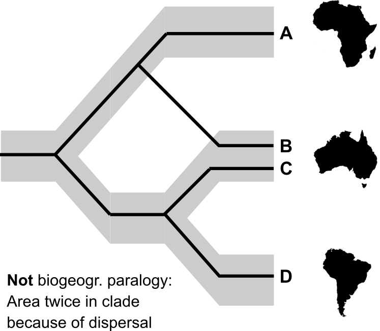
But really crucial is the biogeographic parallel to gene introgression: dispersal. The above scenario shows what area cladists call paralogy and, as we saw in the quotes above, consider evidence of vicariance, but what reason is there to exclude dispersal as a possible explanation? This is, of course, precisely the pattern that dispersal would produce!

And it is clearly not in any way comparable to gene paralogy anyway, because there are no paralogues involved. It makes no sense to use a term that assumes the existence of two genes independently tracing the species phylogeny (and, by analogy, two species-lineages independently tracing 'area relationships') to refer to any difficult pattern, even where there are no such two deep species-lineages.

In summary, I am still not exactly convinced that area cladistics makes sense. The assumption that pretty much any pattern - congruence as well as the contradictory data from paralogy! - is evidence of vicariance seems particularly hard to swallow.